K-function
Tags :: Spatial Statistics
Overview
- A measure of second order dependence
- Gives characteristics of spatial dependence of events across varying scales (i.e. at different spatial distances)
- Assumes 2nd order stationarity and isotropy
Funk
\[ K(h) = \frac{1}{\lambda}E(d_n) \] where \(\lambda\) is the mean number of events per unit area (constant within the domain \(D\)), \(h \geq 0\) is any positive distance (spatial lag), and \(d_n\) is the number of events within distance h of a randomly chosen event}
> Lags will depend on the domain you are analyzing. It is also generally not a good practice to consider lags near the maximum distance across the spatial domain of interest.
Estimating
Estimated as: \[ \hat{K}(h) = \frac{1}{\hat{\lambda}}\frac{1}{N}\sum_{i=1}^{N}\sum_{j=1, j\neq i}\delta(d_{ij} < h) \] where
- \(N\) is the number of events in \(D\)
- \(d_{ij}\) is the euclidian distance between events i and j
- \(\delta(d_{ij} < h) = \begin{cases}1 & \text{ if } d_{ij}<h\\ 0 & \text{ otherwise } \end{cases}\)
- \(\hat{\lambda} = \frac{N(D)}{|D|}\)
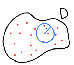
> Visualization of a single \(h\). The polygon will be \(D\).
The inner sum counts the number of events within distance \(h\) of the $i$th event and the outer sum accumulates these counts over all events.
The K-function is biased because of edge effects.
For \(h\) larger than the distance of a particular event to the nearest boundary, the count of events will be too small because events outside the boundary are not counted.
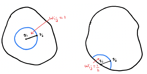
Accounting for edge effects
A weighted sum can be used instead to account for edge effects: \[ \hat{K}(h) = \frac{1}{\hat{\lambda}}\frac{1}{N}\sum_{i=1}^{N}\sum_{j=1, j\neq i}\frac{1}{w_{ij}}\delta(d_{ij} < h) \] where \(w_{ij}\) is the proportion of the circumference of the circle centered at event \(i\) with radius \(d_{ij}\) that lies within the study area.
What should K(h) look like?
If pointss are distributed randomly, then we expect \(\lambda\pi h^2\) within distance \(h\). Therefore,
- \(K(h) = \pi h^2\) for Complete Spatial Randomness
- \(K(h) < \pi h^2\) for regularity (fewer events within distance \(h\) than Complete Spatial Randomness)
- \(K(h) > \pi h^2\) for clustering (more events within distance \(h\) than Complete Spatial Randomness)
Simulating in R
splancs has a built in function to calculate \(\hat{K}\). It requires events, the polygon (spatial domain of interest), and the spatial lags (distances) at which to evaluate the K-function
Start with simulating a homogenous poisson point process with the spatial domain \(X = [-2, 2], Y=[0, 4]\) and an intensity of \(\lambda = 5\).
library(maps)
library(splancs)
set.seed(15)

area <- 4*4
lambda <- 5

N <- rpois(1, lambda * area) # simulate number of points to use
bbox <- as.points(
    c(-2, 2, 2, -2, -2),
    c(0, 0, 4, 4, 0)
)

pts.csr <- csr(bbox, N) # Generate from CSR process
polymap(bbox)
pointmap(pts.csr, add=TRUE)
Using splancs::khat we calculate \(\hat{K}\) from the simulated CSR. We assume we are interested in spatial lags from 0.1 to 2.5 at intervals of 0.1.
h <- seq(0.1, 2.5, 0.1)
kpts <- splacs::khat(pts.csr, bbox, h) # calc K-function

plot(h, kpts, type="l")