Image Transformations
Tags :: Image processing
An image transformation \(T\) can be expressed as
\[ g(x,y)=T[f(x,y)] \]
where \(f(,xy)\) and \(g(x,y)\) are the original and transformed images, repsectively.
Typically \(T\) takes neighbor pixels of \((x,y)\).
If the size of the neighborhood is \(1x1\), \(g\) is a function of \(f\) only. This is also called point processing.
Basic transformations
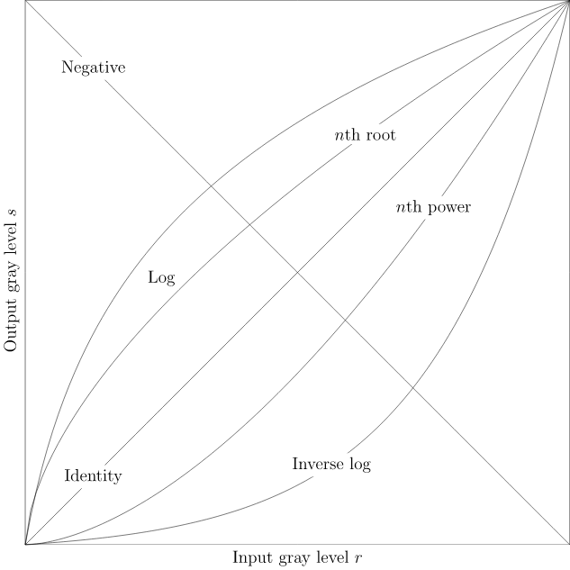
Image negatives
Enhances white or gray detail embedded in dark regions. Separates high and low values into effectively two different domains.
\[ s = L - 1 - r \]
Log transformations
Spreading low \(r\) values, compressing high \(r\) values.
- Emphasizes or brightens dark pixels
- Makes pixel values more managable, \(log(10^6) \to 6\)
\[ s = clog(1 + r) \]
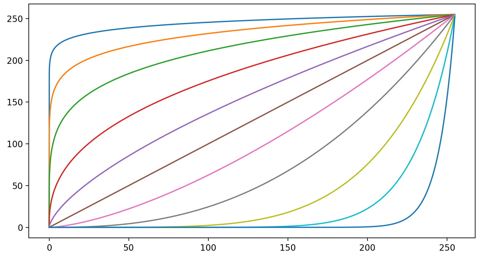
Power-law transformations
Similar to log transformations, but \(\gamma\) controls the overall shape of mapping the curves.
\[ s=cr^\gamma \]
Linear contrast stretching
Essentially making values either dark or white.
\[ T( r)=L_\text{min}+\frac{L_\text{max}-L_\text{min}}{r_\text{max}-r_\text{min}}\times(r-r_\text{min}) \]

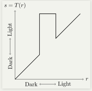
Gray level slicing
Used to highlight a specific range of gray levels, e.g. enhancing water bodies in satellite imagery.
Bit plane slicing
Highlights contributions by specific bits.
Useful to identify which bit planes are significant, to determine the number of bits required, for image compression.