Directly Addressable Codes
Directly Addressable Codes are a type of Compact Data Structure which provides space and time efficient encoding for integer sequences. They obtain a very compact representation if the sequence of integers has a skewed frequency distribution, where the number of occurences of smaller integer values is higher than the number of larger integer values.
Structure
Given a sequence of integers \(X = x_1, x_2, \cdots x_n\), DACs take the binary representation of that sequence and rearrange it into a level shaped structure as follows:
- The first level \(A_1\) contains the first \(n_1\) bits (least significant) of the binary representation of each integer.
- A bitmap \(B_1\) is added to indicate, for each integer, whether its binary representation requires more than \(n_1\) bits or not.
- More precisely, for each integer there is a bit set to 0 if the binary representation of that integer does not need more than \(n_1\) buts and a 1 otherwise.
- In the case of needing more than \(n_1\) bits, the second level \(A_2\) stores the next \(n_2\) bits of the integers having a 1 in \(B_1\), and a bitmap \(B_2\) marks the integers needing more than \(n_1 + n_2\) bits and so on.
This scheme is repeated as many levels as needed, and the number of levels \(\mathcal{L}\) and the number of bits \(n_l\) at each level \(l\), with \(1 \leq l \leq \mathcal{L}\) is calculated in order to achieve maximum compression.
The integer encoded at any give position can be efficiently retrieved by the obtaining the \(n_l\) bits at each level that form the binary representation of the number. I.e. to recover the number a top down traversal is needed and thus the worst cast time for extracting a random codeword is \(O(\mathcal{L})\). The position of the corresponding bits at each level is obtained by performing rank operations over the bitmaps \(B_l\).
If the number of levels and size are adjusted for the number of bits in each level (\(n_l\)) to obtain the maximum possible compression, this may lead to slow access times if it requires a considerable large number of levels. DACs can be configured to obtain the minimum possible space but limiting the number of levels \(L\).
Detailed
Consider an entry \(A[ i ]\) of length \(\ell_i\) . Cut the \(\ell_i\) bits into \(d_i = \lceil\ell_i/b\rceil\) short pieces of \(b\) bits each. Each of the pieces except the last will be prepended with a bit 1, whereas the last will be prepended with a 0. The encoding of \(A[i]\) can then be written as \[ m_{i,1} \cdot p_{i,1} \cdot m_{i,2} \cdot p_{i,2} \cdots m_{i,d_i} \cdot p_{i,d_i} \] where:
- \(p_{i,j}\) - are the pieces
- \(m_{i,j}\) - are the bits prepended to the pieces
The pieces contain the bits of \(A[i]\) from the highest to lowest. I.e. \(A[i]\) is equal to the concatenation \(p_{i,1} \cdot p_{i,2} \cdots p_{i,d}\) , except possible fro some unused highest bits of \(p_{i,1}\). The mark bits are \[ m_{i,r} = \begin{cases} r < d_i \text{ and } m_{i,d_i} = 0, & 1 \\ \text{ otherwise } & 0 \end{cases} \]
The encoding for \(A[1], A[2], \dots, A[n]\) will be stored in a layered way. The first layer stores two arrays:
\begin{align} A_1 & = p_{1,1} \cdot p_{2,1} \cdots p_{n,1}, \\ M_1 & = m_{1,1} \cdot m_{2,1} \cdots m_{n,1} \\ \end{align}
I.e. \(A_1\) stores the first piece of all elements in \(A\) and \(M_1\) stores all the first marking bits. Since all the pieces in \(A_1\) and \(M_1\) are of fixed length (\(b\) and 1, respectively) we can use succinct bit arrays.
Let \(i_1 < i_2 < \dots\) be the elements in \(A\) using more than 1 piece. Our second layer then consists of the following two arrays: $$
\begin{align} A_2 & = p_{i_1,2} \cdot p_{i_2,2} \cdots \\ M_2 & = m_{i_1,2} \cdot m_{i_2,2} \cdots \\ \end{align}
$$ I.e. \(A[2]\) stores the second pieces of all the elements in \(A\) that have 2 or more pieces, and \(M_2\) stores all the corresponding marking bits. This decomposition continues for \(m = \lceil\ell_{\text{max}}/b\rceil\) layers which suffices to represent the longest numbers.
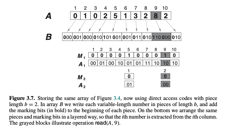
Access
To access \(A[i]\), we start reading \(A_i[1]\) and \(M_1[i]\). if \(M_1[i] = 0\), it means that \(A[i] = A_1[i]\) and the read operation is complete. If instead \(M_1[i] = 1\), then \(A_1[i]\) is only the first piece of a longer element. The problem lies in knowing which is the position \(i’\) that corresponds to \(i\) in \(A_2\). We see that \[ i’ = \sum_{j=1}^iM_1[j] = \text{sum}(M_1, i) \] or equivalently, \(i’\) is the number of 1s in \(M_1[1, i]\). Therefore the bit arrays \(M_r\) are preprocessed for partial sum queries.
Once we obtain \(i’\) from \(i\), we read \(A_2[i’]\) and \(M_2[i’]\). if \(M_2[i’] = 0\) it means that \(A[i]\) spans two pieces, which we have already read, thus we can return \(A[i] = A_1[i] \cdot 2^b + A_2[i’]\). Otherwise, \(M_2[i’] = 1\) and we must continue with \(A_3[i’’]\) and \(M_3[i’’]\) for \(i’’ = \text{sum}(M_2, i’)\) and so on.